This page is a minimal version of our paper arxiv:2112.01288.

How to quantify textures?

To extract information from a stochastic field, we need some vocabulary to describe its statistical properties, i.e., the textures in the field. However, quantifying textures is in general challenging. The most widely used vocabulary – the power spectrum – is concise and easy to use, but has limited ability to characterize complex strucutres, as shown in the figure below. Recently, convolutional neural networks (CNN) have shown impressive ability to perform this task. However, training a CNN involves optimization of millions to billions of parameters and a large training dataset. It also face interpretability and transparency problems, which is crucial for scientific research. What makes CNN so powerful? Is it possible to combine the advantages of both analytical statistics and CNNs?

The scattering transform

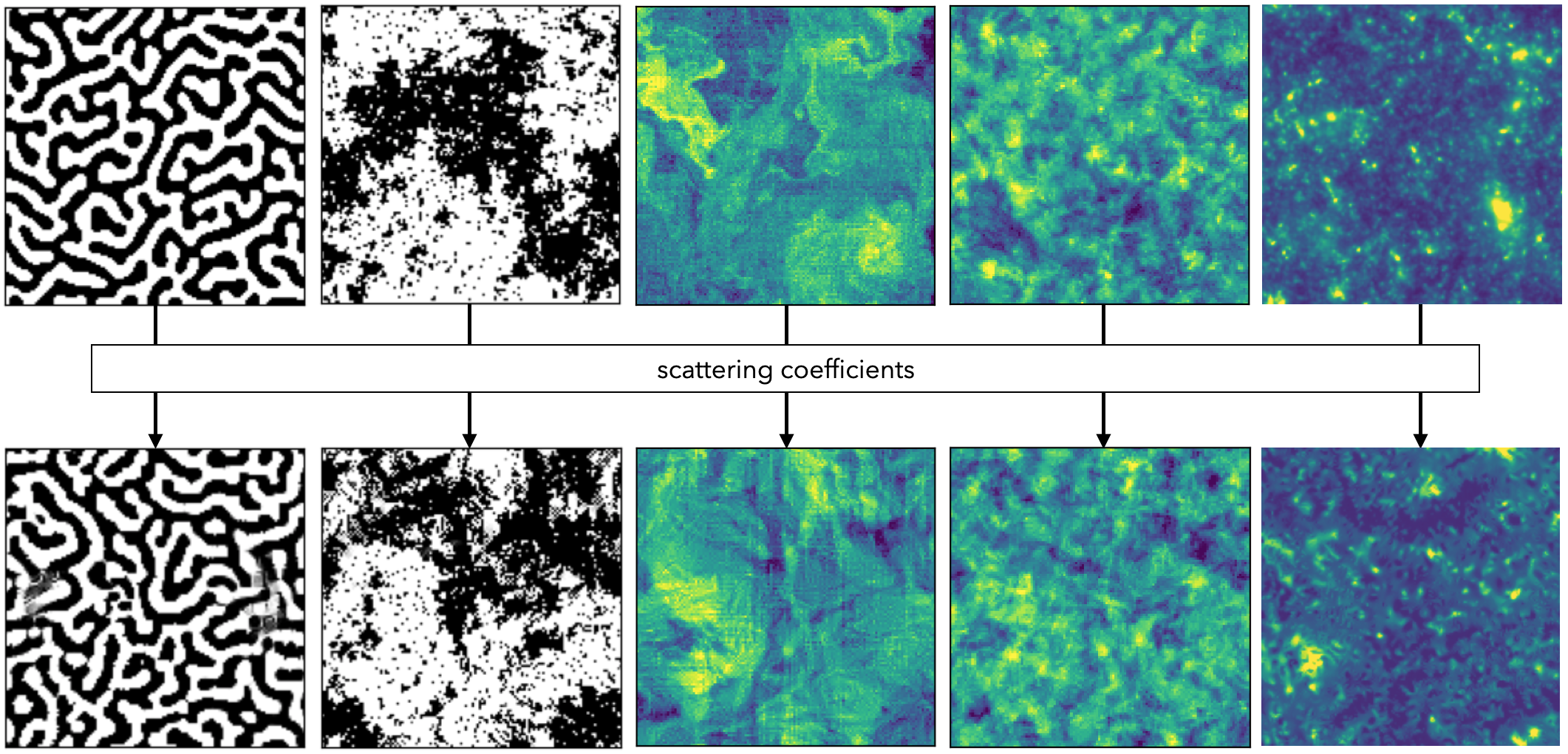
The scattering transform is a statistical tool borrowing ideas from CNNs. On the one hand, it generates a compact set of powerful summary statistics with desirable mathematical properties. On the other hand, it can be seen as a toy-model for CNNs with pre-determined filters, and can be used to decipher the inner working of CNNs. To demonstrate its power, we show image synthesis result on a variety of physical fields using the scattering transform (see the figures above and below). Image synthesis is a way to visualize what a field looks like in the eye of a particular statistic. The textural similarity between the inputs and synthesis results reveals the informativeness of the scattering statistics. For more details, please see our paper.

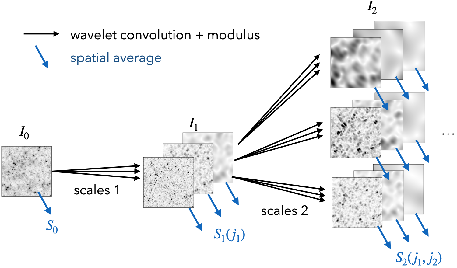
An illustration of the definition of the scattering transform is shown in the figure below. It transforms the input field by wavelet convolutions and pointwise non-linearity (complex modulus) and repeats this combination of operations to go higher orders. Then, to obtain translation-invariant statistics, it takes the global average of the respective transformed fields. They are called `scattering coefficients’. Its structural similarity to CNNs can be clearly seen in the figure below.

Interpretation

The scattering transform has very interesting visual interpretation. The first-order scattering coefficients are similar to binned power spectrum. Indeed, if we raise the modulus operation into squared modulus, these coefficients becomes exactly the binned power spectrum.

The second-order scattering coefficients are more interesting, as they contain substantial non-Gaussian information and can also be interpreted. After a further reduction, these coefficients can represent the sparsity and shape of features in the field:


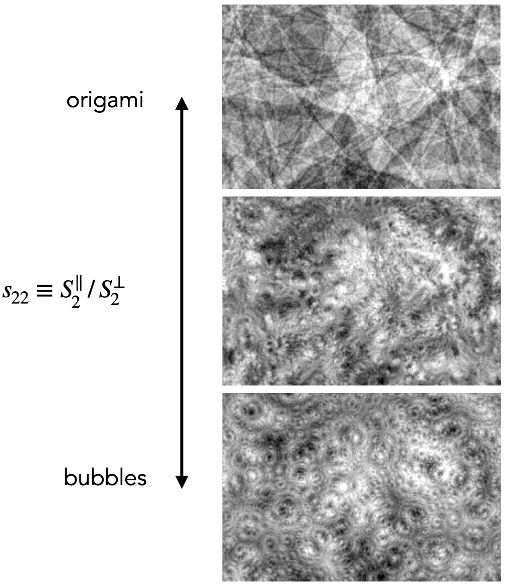
More visualization can be found here.

Applications

Given the vocabulary and data representation provided by the scattering transform, one can use it in a wide variety of applications, from data exploration (outlier detection, similarity estimate, etc) to classifications and parameter inference.

For data exploration, we are working on its application to oceanography data, where it shows great promises. For example, by simple compressing the scattering coefficients into two numbers (averaged sparsity and shape in all scales), the sea surface temperature cutouts can be meaningfully arranged, as shown below. Interestingly, there are some the big, rare eddies in the dataset, which are easily recognized at the very bottom of this scattering transform representation, but missed by a CNN + normalizing flow outlier detector in another analysis.

For classifications, one possible application in astronomy is on galaxy morphology.

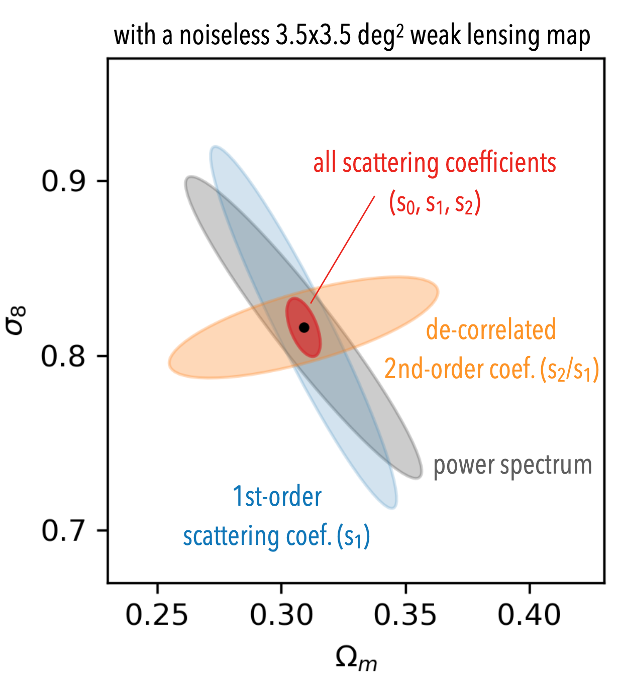
For parameter inference, we have two papers on cosmological parameter inference, where its performance is on a par with state-of-the-art CNNs ([1], [2]).

Contacts

scheng@ias.edu
+1 443 207 1532
Institute for Advanced Study
Princeton, NJ 08540, USA